Once a Thermoptim model is finalized, its diagram and project files contain all the information needed for its complete resolution. It is therefore possible to use them to generate the corresponding set of equations, thanks to a feature of the software currently under development.

This allows, in particular:

• To maintain a systemic approach in describing the architecture of the model, while providing access to its equations, so that they can be used in other environments and additional processing can be performed beyond what the software offers, such as optimization.

• To ensure the consistency of the sets of equations for large-scale models, which can be difficult in practice if an appropriate tool is not available.

• Thermoptim can thus be used as a preprocessor for various applied thermodynamics solvers, such as Interactive Thermodynamics, EES, or Matlab.

The following conventions are used:

• The names of unknowns are defined by concatenating their usual symbol (T, p, h, s, v...) with the name of the point or process, using the underscore ‘_' as a link. Thus, the enthalpy of point 2 is written as h_2. The advantage of this notation is that it is very clear, and it transforms into h2 if the equation is displayed in editors using LaTeX syntax. Note that you can add variables and equations to have them analyzed by Thermoptim. In this case, the variable names must contain the underscore to be taken into account, and each new equation must be preceded by the line //Equation: ijk, ijk being its number.

• Flow rates are denoted as ‘m_dot_' followed by the name of the process, for example, m_dot_condenser for the flow rate that passes through the process ‘condenser'.

• When special characters or spaces are used in the names of Thermoptim elements, they are simply removed. For example, the enthalpy of the point ‘entrée d'air' will be written as h_entredair. Nothing prevents renaming this unknown later if desired.

• The functions for calculating properties are generated in two steps. They are first written in the following generic format, which is easy for a human to interpret: functionName("fluid";T = T_1;P = P_1). The arguments of the function are thus clearly identifiable, without risk of permutation. Thus, the calculation of the enthalpy of water knowing its pressure and entropy is written as: calcH_PS("eau";P = p_2;s = s_2).

• The equation set thus generated can then be easily converted to the specific format of each solver.

• Comments can be added either on a complete line or after an equation. They are preceded by the characters ‘//', according to the syntax used in a number of programming languages.

• It should be noted that it is not intended to provide equations for all the numerous parameterizations that Thermoptim allows because, once a set of equations is established, it is easy to modify some of them manually according to the objectives pursued. For example, the equation chosen to calculate the output pressure of a compressor can be the product of the input pressure by the known compression ratio. It remains valid if the pressure is set and the compression ratio is calculated. To change the parameterization, it is sufficient to change the known value.

• Since a heat exchanger or a combustion chamber is generally isobaric, we have implemented P_downstream = P_upstream.

• In the entry process-points, the complete state is calculated as given value, as well as the flow rate.

• To determine the flow rates, we start from the process with set flow rates or those downstream of the nodes, which are all recalculated, and we propagate the flow rate to those downstream if the connection is unique.

• Although this is not a mandatory requirement for most solvers, the equations are generally written in the form “Variable = expression as a function of other variables”.

Currently, the formal generation of equations is only implemented for the core components of Thermoptim, and this implementation remains provisional. Therefore, some modifications in the generated files are to be expected in the future.

The equations generated for a turbine modeled with an isentropic reference and a given expansion ratio are of the following type:

//Process: turbine

//Equation : 23

m_dot_turbine = m_dot_superheater // Upstream process : superheater - Downstream process : turbine

//Equation : 24

s_3 = calcS_PH("water";P = p_3;H = h_3) // Upstream point : 3 - Downstream point : 4

// Comment = Isentropic reference

//Equation : 25

hs_4 = calcH_PS("water";P = p_4;S = s_3) // Downstream point : 4

//Equation : 26

etaT_turbine = 0.9// Isentropic efficiency

//Equation : 27

h_4 = h_3 - etaT_turbine*(h_3 - hs_4) // Upstream point : 3 - Downstream point : 4

//Equation : 28

xl_4 = 0.// Saturated liquid quality

//Equation : 29

Tl_4 = T_4- 0.01// Saturated liquid temperature

//Equation : 30

xv_4 = 1.// Saturated vapor quality

//Equation : 31

Tv_4 = T_4+ 0.01// Saturated vapor temperature

//Equation : 32

hl_4 = calcH_TPx("water";T = Tl_4;P = p_4;X = xl_4)// Saturated liquid enthalpy

//Equation : 33

hv_4 = calcH_TPx("water";T = Tv_4;P = p_4;X = xv_4)// Saturated vapor enthalpy

//Equation : 34

x_4 = (h_4 - hl_4)/(hv_4 - hl_4)// Quality

//Equation : 35

T_4 = calcTsat("water";P = p_4 ;X = x_4) // Downstream point : 4

//Equation : 36

s_4 = calcS_PH("water";P = p_4;H = h_4) // Entropy

// Comment = Given outlet pressure

//Equation : 37

p_4 = 0.0356// Outlet pressure

//Equation : 38

W_dot_turbine = m_dot_turbine*(h_4 - h_3) // DeltaH

Equation 23 translates the propagation of the flow rate from the upstream process.

Equation 24 calculates the entropy of the upstream point, and Equation 25 calculates the enthalpy of the downstream point corresponding to the isentropic evolution.

Equation 26 provides the value of the isentropic efficiency, and Equation 27 determines the actual enthalpy of the downstream point.

Equations 28 to 34 provide the turbine outlet quality.

Equation 35 provides the temperature of the downstream point, and Equation 36 provides its entropy.

Equation 37 gives the downstream pressure, and Equation 38 gives the useful work.

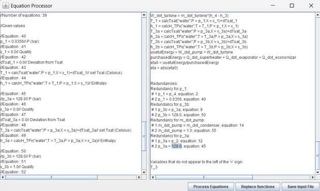
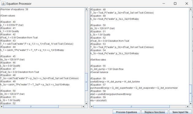
Thermoptim automatically extracts from the model a first set of commented equations that can be considered raw. Their number is quite high, as a process typically requires more than a dozen: 4 for the state of each entry and exit point (T, p, x, h), 2 for the flow rate and the energy involved delta H, plus those allowing its calculation.

Even a very simple model generally includes at least fifty such equations.

Analyzing this set of raw equations to verify their consistency and identify any gaps can be a tedious task if done manually.

Utilities are available to facilitate this process.

The first step consists of resolving the redundancies that may exist between the equations, particularly when a variable is calculated in two different ways, which can occur depending on the model's parameterization. The analysis that is carried out considers that there is redundancy if the same variable x_y appears twice to the left of the '=' sign: x_y = expression 1, x_y = expression 2.

These redundancies are caused by variants in the interpretation of the Thermoptim model parameterization. Since the software is not capable of choosing between the concerned equations, it is up to the modeler to do so, especially since some apparent redundancies are not true redundancies, as some variables may have to be calculated by inverting one or more equations.

Thermoptim establishes a list of potential redundancies, and it is up to the user to remove the unnecessary equations by comparing those that have been generated and retaining those they desire. To do this, the user simply double-clicks on a redundancy line to add or remove '//' in front of the equation, which disables or enables the equation. The same '//' appears on the selected line in the right screen, to remind you that it has been changed.

The choice between redundant equations is not always straightforward. To help you choose, you can display them successively in the left screen by double-clicking on each of them, which allows you to know which block it belongs to and to consult the comments that accompany it. Don't forget to double-click a second time to revert to the previous state of the equation until you have made your final selection.

The second step allows for signaling if a variable in the problem never appears on the left side of an equation, which a priori suggests that it is neither initialized nor calculated from one of the equations. This allows for detecting potential oversights in the definition of the problem to be solved. An example is that of a simple steam cycle, where the turbine inlet temperature is not automatically considered by Thermoptim as a given value.

However, as with redundancies, some variables do not appear explicitly to the left of the '=' sign in the equations, because they are calculated by inverting some of them. To potentially reduce the dimension of the problem, an algorithm for ordering the remaining equations has been developed and can be used in a third step.

Its principle is as follows:

It begins by identifying all variables that Thermoptim considers to have set values, with the generated equation in the form "Variable = numerical data".

For example:

m_dot_condenser = 100 // Set flow

This provides a first group of resolved equations that correspond to the problem's data.

The second group consists of equations that depend only on the variables of the first group.

For example:

m_dot_feedpump = m_dot_condenser // Flow propagation

A third group is one whose equations depend only on the variables of the first and second groups, and so on, with the algorithm operating recursively.

At the end, there remains a group of equations to be solved using the solver, with the solutions of the others being directly obtainable by substituting the unknown variables with those already calculated.

The presentation of the procedure for reducing the model size can also have a didactic interest.

Of course, this ordering is unnecessary if the solver is powerful and used blindly.

As already indicated, the number of Thermoptim parameters is very high. It would be difficult to predict all the corresponding equations, but this would not be of great interest anyway, given that once a set of equations is validated, it is very simple to complete it at will according to the objectives pursued. Therefore, only the main parameterizations have been retained.

Direct dependency graph

An additional feature has been added to the analysis of the equation set generated by Thermoptim.

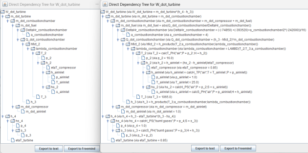
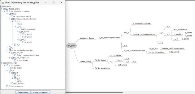
When a variable is one of the groups highlighted above, it is possible to display the graph of its direct dependencies on those of the lower rank groups. To do this, simply select it in the left panel of the equation processor screen, then click on the "Display dependency graph" button. The Direct Dependency Tree is displayed in two forms in two new windows, which allow it to be exported in text or mind map format. One of the windows simply displays the graph of the dependent variables, while the other additionally displays the equations that determine this dependence, as shown in the figure below.

Note that the analysis of the equations is done on the entire content of the left panel and not only on the equations generated by Thermoptim. Provided, of course, that it follows the same format as these, you can use these features on any set of equations.

Note also that this type of graph can only be established for variables that can be computed directly from the other variables in the lower-ranked groups. Variables that can only be calculated by solving the group of unresolved equations cannot be considered.

Exporting to Freemind format allows the dependency tree to be kept as a mind map.

As mentioned earlier, the property calculation functions initially generated by Thermoptim are written in the following generic format, which is easy for a human to interpret: functionName("fluid";T = T_1;P = P_1). The arguments of the function are thus clearly identifiable, without risk of permutation. For example, the calculation of the enthalpy of water knowing its pressure and entropy is written as: calcH_PS("water";P = p_2;s = s_2).

It is therefore necessary to convert them to the specific format of the server you wish to use. For example, in Interactive Thermodynamics, this last expression must be written in the form h_Ps("water", p_2, s_2), and in EES as enthalpy(Steam;P= p_2;s = s_2).

It is also important to verify the unit parameterization in the solver. For Thermoptim, it is the SI system, with pressures expressed in bar and temperatures in °C. The unit of flow rates is indicated before the equations.

Once the set of equations is deemed satisfactory, it must be converted into the syntax of the particular solver that will be used.

Composition of Compound Gases

The two solvers for which the process of converting the generated equations has been implemented so far are Interactive Thermodynamics et EES.

I encountered difficulties in converting the calculation of the properties of compound gases from Thermoptim to these two solvers due to the inability, to my knowledge (admittedly limited), to define a new compound gas and calculate its thermodynamic properties. For EES, I saw that solutions exist, but I do not know how to automate them from Thermoptim files. For Interactive Thermodynamics, I did not see how to do it.

This means that the equations for systems involving such fluids cannot be fully generated by Thermoptim, except for a few gases like air, which is actually treated as a pure gas. Modelers will need to complete them with specific functions that they will have to code. In order to facilitate this task, the composition of these compound gases is indicated in the generated file in the form of comment lines, as shown in this example:

//GAS COMPOSITIONS

//burnt_gas

//CO2 0.04419006337631066

//H2O 0.03617814048485812

//O2 0.1640556604215191

//N2 0.7433597848138069

//Ar 0.012216350903505186

//air

//N2 0.7555302216468832

//Ar 0.012416359476160373

//O2 0.2320534188769565

//CH4 ` methane

//CH4 ` methane 1.0

Combustion chambers

The generation of equations corresponding to combustion chambers is particularly complex due to the number of possible parameterization options and the determination of the composition of the burned gases.

Given these difficulties, I opted for a provisional solution that allows combustion to be performed in EES, thereby enabling the study of cycles such as gas turbines or internal combustion reciprocating engines involving only a single combustion with air as the oxidizer and methane (CH4) as the fuel. This solution can serve as a first step before developing more detailed combustion models.

The reaction is assumed to be complete. Its equation is:

Lambda is the air factor, and a is the number of hydrogen atoms per carbon atom. In this case, a = 4 for methane.

When the studied system includes a combustion chamber, the beginning of the generated file contains three EES functions that allow the estimation of:

• the air factor of the combustion as a function of the oxidizer temperature and the desired adiabatic combustion temperature, as well as the value of a for a fuel of type CHa

• the enthalpy of the combustion products as a function of their temperature, the air factor, and a

• the entropy of the combustion products as a function of their temperature and pressure, the air factor, and a

With the upstream and downstream points being 2 and 3, the block of equations corresponding to a combustion chamber is of the type:

//Process: combustion chamber

// Comment = Calculate lambda simplified model oxidizer air, fuel CH4

//Equation: 28

T_3 = 1065.0// Given value (Celsius)

//Equation: 29

a_combustionchamber = 4// for CH4

//Equation: 30

lambda_combustionchamber = LAMBD(T_2;T_3;a_combustionchamber)// air factor lambda

//Equation: 31

h_3 = h_products(T_3;a_combustionchamber;lambda_combustionchamber)// enthalpy of the reactants

//Equation: 32

hfict_2 = h_products(T_2;a_combustionchamber;lambda_combustionchamber)// enthalpy of a fictitious inlet point for calculating the heat released

//Equation: 33

m_dot_combustionchamber = m_dot_compressor + m_dot_fuel // Upstream process - compressor - Fuel process fuel - Downstream process - combustion chamber

//Equation: 34

//m_dot_turbine = m_dot_combustionchamber //Flow propagation

//Equation: 35

Q_dot_combustionchamber = (h_3 - hfict_2)*m_dot_combustionchamber // DeltaH

//Equation: 36

DeltaHr_combustionchamber = (-(-74850) +(-393520)+a_combustionchamber/2*(-242000))/16 // DeltaHr (kJ/kg) = (-(-74850) +(-393520) + a/2* (-242000))/16 for methane

//Equation: 37

m_dot_fuel = Q_dot_combustionchamber/DeltaHr_combustionchamber // fuel flow rate

// Comment = Isobaric process

//Equation: 38

p_3 = p_2// Isopressure

//Equation: 39

T_fuel = 15.0// Given value (Celsius)

//Equation: 40

p_fuel = 20.0// Given value (bar)

//Equation: 41

h_fuel = calcH_TP("CH4 ` methane";T = T_fuel ;P = p_fuel) // Fuel point - fuel

Equation 28 sets the value of the desired adiabatic 00combustion temperature, equation 29 sets the value of a, and equation 30 calls the EES function that provides lambda.

Equation 31 calculates the enthalpy of the gases exiting the combustion chamber. It is important to note a significant problem encountered at this stage: I could not find the reference value h0 for the enthalpies of the burned gases to make them comparable to those of other fluids. There is therefore a discrepancy between these two sets of properties. This only poses a problem at the level of the combustion chamber itself.

This is why the fictitious enthalpy hfict_2 is introduced in equation 32. It allows us to know the value of the enthalpy of the upstream point calculated with the composition and equations of the downstream point.

Equation 33 ensures the conservation of flow. Equation 34 was nullified because it was redundant and different.

Equation 35 determines the heat released during combustion, using hfict_2 introduced previously.

Equation 36 calculates the reaction enthalpy of the combustion equation, and equation 37 uses it to determine the required fuel flow rate.

Equation 41 calculates the enthalpy of the fuel. The name of its substance needs to be modified to become CH4.

Calculations Downstream of a Combustion Chamber

The calculations downstream of the combustion chamber require special treatment because the burned gases are not recognized as a substance by the solvers. The determination of their properties is done using two of the three introduced EES functions, which provide enthalpy and entropy but do not invert these functions.

Given that the calculation of the thermodynamic properties of the burned gases cannot be performed with the usual functions, it is necessary to replace all calls to these functions for the Thermoptim substance that represents them with their equivalent defined in the EES functions placed at the beginning of the generated file. This does not pose any particular difficulty for calculations linking h and s to T and p, but it is more delicate for those directly relating h and s, which assume inversions of these functions.

Therefore, one is led to slightly reformulate the problem depending on the situation, as illustrated by the calculation of a turbine calculated in polytropic reference mode presented below, where only the equations for calculating properties need to be modified. The upstream point is 3 and the downstream point is 4.

It should be noted that lines starting with // are comment lines that the solver does not take into account.

//Process: turbine

// Comment = Polytropic coefficient: k = -Math,log(aval,p/amont,p)/Math,log(aval,V/amont,V)

//Equation: 24

//h_4 = enthalpy(burnt gases;P = p_4;S = s_4) // Enthalpy

h_4 = h_products(T_4;a_combustionchamber;lambda_combustionchamber)// enthalpy of the reactants

//Equation: 25

//T_4 = temperature(burnt gases;H = h_4) // Downstream point - 4

s_4 = s_products(T_4;p_4;a_combustionchamber;lambda_combustionchamber)// enthalpy of the reactants

Equations 24 and 25 are replaced as follows: the calculation of h_4 as a function of T_4 (unknown), is provided by the solver's inversion of the equation giving s_4 (known) as a function of T_4.

As can be seen, in this case, it is necessary to slightly reformulate the problem.

For an isentropic expansion, here is a slightly more complex example of reformulation:

//Equation: 18

//s_3 = entropy(burnt gases;P = p_3;H = h_3) // Upstream point - 3 - Downstream point - 4

s_3 = s_products(T_3;P_3;a_combustionchamber;lambda_combustionchamber)

// Comment = Isentropic reference

//Equation: 19

//hs_4 = enthalpy(burnt gases;P = p_4;S = s_3) // Downstream point - 4

hs_4 = h_products(Tis;a_combustionchamber;lambda_combustionchamber)

s_3 = s_products(Tis;P_4;a_combustionchamber;lambda_combustionchamber)

//Equation: 20

etaT_turbine = 0,85// Isentropic efficiency

//Equation: 21

h_4 = h_3 - etaT_turbine*(h_3 - hs_4) // Upstream point - 3 - Downstream point - 4

//Equation: 22

//T_4 = temperature(burnt gases;H = h_4) // Downstream point - 4

h_4 = h_products(T_4;a_combustionchamber;lambda_combustionchamber)

//Equation: 23

//s_4 = entropy(burnt gases;P = p_4;H = h_4) // Entropy

s4 = s_products(T_4;P_4;a_combustionchamber;lambda_combustionchamber)

Equation 18 is a simple reformulation of the one generated.

To solve equation 19, we introduce the isentropic temperature Tis, which is determined from the function giving the known enthalpy, and the equation giving the enthalpy from Tis provides the isentropic enthalpy.

Equations 22 and 23 are simple reformulations of the ones generated.

Three commented examples are provided in these pages, with the corresponding equation files, as well as others uncommented.

• Steam Power Plant Cycles

• Refrigeration Cycle

• Gas Turbine Cycles

• Combined Cycles