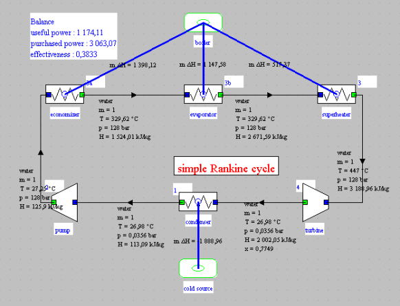
It is a very simple cycle, the synoptic view of which is given below:

The diagram and project files are given below. Please note that they require the use of Thermoptim in English, i.e. with the inth2.zip file of this language.

There are 54 of them. They are given in this file.

There is no redundancy identified.

The algorithm detects that there is a missing piece of information for the problem to have a solution, which is consistent with the fact that there are only 53 variables.

Variables that do not appear to the left of the '=' sign:

T_3

T_3 is not provided, although it is the superheat temperature, which is a given value that cannot be deduced from other parameters. Therefore, it will need to be added to the list of final equations.

Once the missing equation is added, the analysis of the equations can be started again. It makes it possible to highlight the different groups of equations that can be solved simply.

Group 1

Group 1 (14 Variables) : [dTsat_1, x_3b, p_2, x_3a, p_4, m_dot_pump, T_3, xv_4, x_1, etaT_pump, etaT_turbine, xl_4, dTsat_3b, dTsat_3a]

Group 1 (Equations):

etaT_pump = 1.0

p_2 = 128.0

etaT_turbine = 0.9

xl_4 = 0.

xv_4 = 1.

p_4 = 0.0356

x_1 = 0.0

dTsat_1 = 0.0

x_3a = 0.0

dTsat_3a = 0.0

x_3b = 1.0

dTsat_3b = 0.0

m_dot_pump = 1.0

T_3 = 447

We find here all the equations providing the data for the problem, including T_3.

Group 2

Group 2 (3 Variables) : [m_dot_economizer, p_1, p_3a]

Group 2 (Equations):

p_1 = p_4

m_dot_economizer = m_dot_pump

p_3a = p_2

This second group corresponds to equations that allow the calculation of new variables through simple substitution of those from the first group.

Group 3

Group 3 (4 Variables) : [m_dot_evaporator, T_1, p_3b, T_3a]

Group 3 (Equations):

m_dot_evaporator = m_dot_economizer

p_3b = p_3a

T_1 = calcTsat("water";P = p_1;X = x_1)+dTsat_1

T_3a = calcTsat("water";P = p_3a;X = x_3a)+dTsat_3a

This third group corresponds to equations that allow the calculation of new variables through simple substitution of those from the first and second groups.

The process is repeated in the subsequent groups.

Finally, we obtain the following list of unresolved equations:

Unresolved Equations: 14

Q_dot_economizer = m_dot_economizer*(h_3a - h_2)

v_2 = calcV_PH("water";P = p_2 ;H = h_2)

h_2 = h_1 + v_2*(p_2 - p_1)/100.

T_2 = calcT_PH("water";P = p_2 ;H = h_2)

W_dot_pump = m_dot_pump*(h_2 - h_1)

Tl_4 = T_4- 0.01

Tv_4 = T_4+ 0.01

hl_4 = calcH_TPx("water";T = Tl_4;P = p_4;X = xl_4)

hv_4 = calcH_TPx("water";T = Tv_4;P = p_4;X = xv_4)

x_4 = (h_4 - hl_4)/(hv_4 - hl_4)

T_4 = calcTsat("water";P = p_4 ;X = x_4)

useful_Energy = W_dot_pump + W_dot_turbine

purchased_Energy = Q_dot_superheater + Q_dot_evaporator + Q_dot_economizer

eta_global = abs(useful_Energy/purchased_Energy)

These are the equations that either depend on the properties of the fluid or cannot be directly solved.

The 14 missing variables are also identified.

Interactive Thermodynamics is a solver provided by MM. Moran, Shapiro and Mmes Boettner and Bailey as a supplement to their book "Fundamentals of Engineering Thermodynamics, 8th Edition", which can be downloaded freely.

The conversion allows for obtaining a file that can be processed by the solver.

The equations for calculating fluid properties converted to this format are given below, with the others remaining unchanged:

//Equation: 6

h_3 = h_PT("water",p_3,T_3)// Enthalpy

//Equation: 14

s_1 = s_Ph("water",p_1,h_1) // Upstream point - 1 - Downstream point - 2

//Equation: 15

hs_2 = h_Ps("water",p_2,s_1) // Downstream point - 2

//Equation: 17

v_2 = v_Ph("water",p_2,h_2) // Downstream point volume -

//Equation: 18

h_2 = h_1 + v_2*(p_2 - p_1)/100. // Liquid compression

//Equation: 19

T_2 = T_Ph("water",p_2,h_2) // Downstream point - 2

//Equation: 23

s_3 = s_Ph("water",p_3,h_3) // Upstream point - 3 - Downstream point - 4

//Equation: 24

hs_4 = h_Ps("water",p_4,s_3) // Downstream point - 4

//Equation: 26

h_4 = h_3 - etaT_turbine*(h_3 - hs_4) // Upstream point - 3 - Downstream point - 4

//Equation: 31

hl_4 = hsat_Px("water",p_4,xl_4)// Saturated liquid enthalpy

//Equation: 32

hv_4 = hsat_Px("water",p_4,xv_4)// Saturated vapor enthalpy

//Equation: 34

T_4 = Tsat_P("water",p_4) // Downstream point - 4

//Equation: 35

s_4 = s_Ph("water",p_4,h_4) // Entropy

//Equation: 40

T_1 = Tsat_P("water",p_1)+dTsat_1// set Tsat (Celsius)

//Equation: 41

h_1 = hsat_Px("water",p_1,x_1)// Enthalpy

//Equation: 44

T_3a = Tsat_P("water",p_3a)+dTsat_3a// set Tsat (Celsius)

//Equation: 45

h_3a = hsat_Px("water",p_3a,x_3a)// Enthalpy

T_3b = Tsat_P("water",p_3b)+dTsat_3b// set Tsat (Celsius)

//Equation: 49

h_3b = hsat_Px("water",p_3b,x_3b)// Enthalpy

The file that can be solved in Interactive Thermodynamics is provided below.

EES is a solver developed by f-Chart, which requires a license. The conversion results in a file that can be processed by the solver. The equations for calculating the fluid properties converted to this format are given below, the others remaining unchanged:

//Equation: 6

h_3 = enthalpy(Water;P = p_3;T = T_3)// Enthalpy

//Equation: 14

s_1 = entropy(Water;P = p_1;H = h_1) // Upstream point - 1 - Downstream point - 2

//Equation: 15

hs_2 = enthalpy(Water;P = p_2;S = s_1) // Downstream point - 2

//Equation: 17

v_2 = volume(Water;P = p_2;H = h_2) // Downstream point volume -

//Equation: 18

h_2 = h_1 + v_2*(p_2 - p_1)/100, // Liquid compression

//Equation: 19

T_2 = temperature(Water;P = p_2;H = h_2) // Downstream point - 2

//Equation: 23

s_3 = entropy(Water;P = p_3;H = h_3) // Upstream point - 3 - Downstream point - 4

//Equation: 24

hs_4 = enthalpy(Water;P = p_4;S = s_3) // Downstream point - 4

//Equation: 26

h_4 = h_3 - etaT_turbine*(h_3 - hs_4) // Upstream point - 3 - Downstream point - 4

//Equation: 31

hl_4 = enthalpy(Water;P = p_4;X = xl_4)// Saturated liquid enthalpy

//Equation: 32

hv_4 = enthalpy(Water;P = p_4;X = xv_4)// Saturated vapor enthalpy

//Equation: 34

T_4 = t_sat(Water;P = p_4) // Downstream point - 4

//Equation: 35

s_4 = entropy(Water;P = p_4;H = h_4) // Entropy

//Equation: 40

T_1 = t_sat(Water;P = p_1)+dTsat_1// set Tsat (Celsius)

//Equation: 41

h_1 = enthalpy(Water;P = p_1;X = x_1)// Enthalpy

//Equation: 44

T_3a = t_sat(Water;P = p_3a)+dTsat_3a// set Tsat (Celsius)

//Equation: 45

h_3a = enthalpy(Water;P = p_3a;X = x_3a)// Enthalpy

//Equation: 48

T_3b = t_sat(Water;P = p_3b)+dTsat_3b// set Tsat (Celsius)

//Equation: 49

h_3b = enthalpy(Water;P = p_3b;X = x_3b)// Enthalpy

The file that can be resolved in EES is provided below.

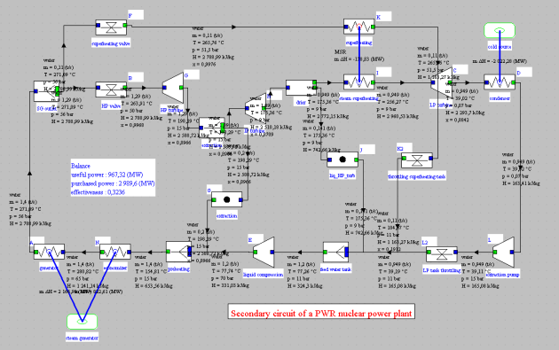
PWR nuclear reactor cycle with extraction

Raw Equations File (175 Equations)

Executable file in IT

Executable file in EES